algbio-edu
algbio-edu — interactive visualizers for algorithmic bioinformatics
Want a new visualization? Open an issue and describe the algorithm — contributions and requests are welcome.
Single-page web demos for the central algorithms taught in an “Algorithmic Bioinformatics” course (FU Berlin ALBI, WS 2024 lectures by Hölzer / Backofen / Liebl). Each demo follows the same pattern:
- a DP matrix (or trellis) heatmap that fills step-by-step,
- a Reset / ◀ Back / Play / Next ▶ controller,
- keyboard shortcuts (← / → / space),
- an output panel showing what the algorithm decoded (alignment / state path / structure).
This is a sister repo to rna-folding-edu (Nussinov + Zuker for RNA secondary-structure prediction).
What’s here
| Folder | Algorithm | Demo |
|---|---|---|
hmm/ |
Viterbi, Forward, Backward, Posterior on a 2-state CpG-island HMM | open |
alignment/ |
Needleman-Wunsch (global) and Smith-Waterman (local) | open |
fm-index/ |
FM Index: BWT construction, reverse transform, backward search, locate matches | open |
evoformer/ |
3-D voxel walk through one Evoformer block (AlphaFold) | open |
structure-scores/ |
GDT-TS / TM-score / lDDT — sliders + intuition | open |
phylo/ |
Neighbor-Joining + UPGMA + Fitch + Sankoff (Python + step-by-step PNG figures) | browse |
For RNA structure (Nussinov + Zuker + 3D PDB): r-sayar/rna-folding-edu (open). For HMM training/evaluation on real DNA (the algorithm code that the HMM viz here visualises): r-sayar/cpg-island-hmm.
Each demo, in one paragraph
HMM inference — hmm/
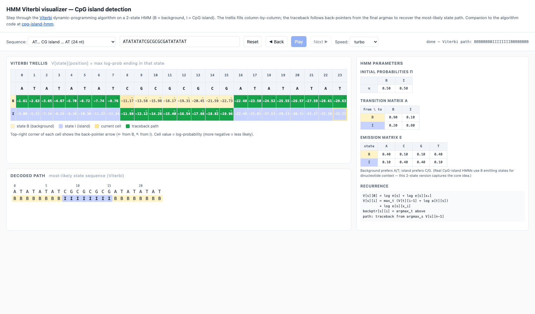
A two-state Hidden Markov Model (B = background, I = CpG island) with hand-tuned emission and transition probabilities, four algorithms selectable from a single dropdown:
- Viterbi — max-product. The trellis fills column-by-column; each
cell stores the max log-prob of any path ending in
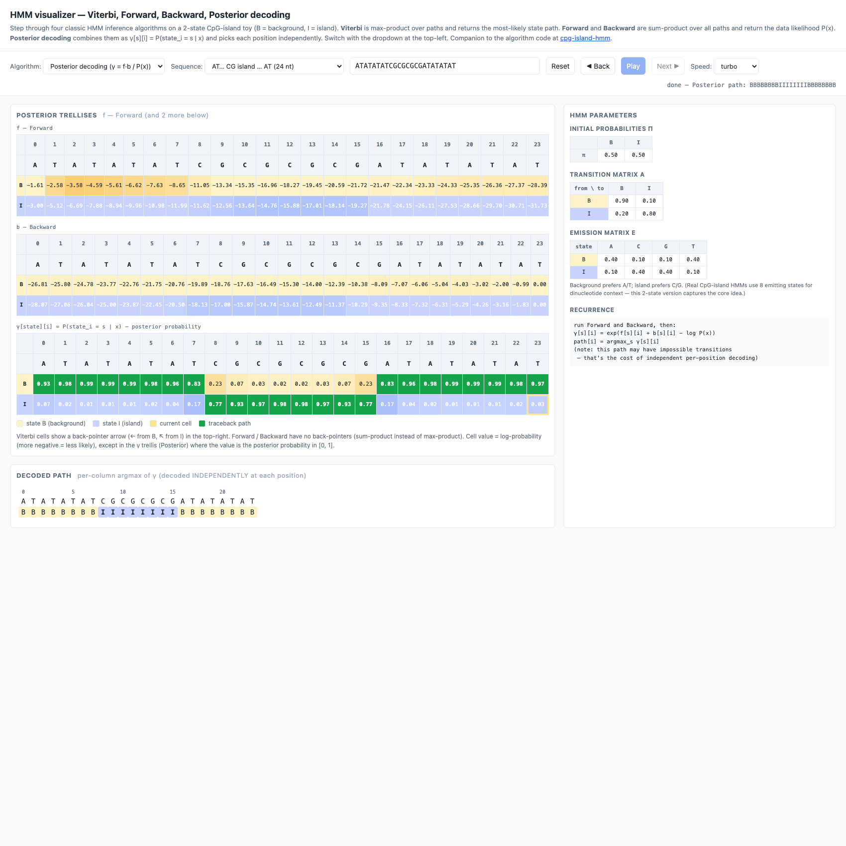
(state, position)plus a back-pointer. The traceback follows back-pointers from the final argmax to recover the single most-likely state path. - Forward — sum-product (logsumexp). Same trellis shape but the
recurrence sums over all paths instead of maxing over them. Output:
log P(x) = logsumexp_s f[s][n-1]. - Backward — sum-product, right-to-left.
b[s][i] = P(x_{i+1}..x_n | state_i = s). Independent recurrence, but should agree with Forward onP(x)— a built-in correctness check. - Posterior decoding — runs both Forward and Backward, then
γ[s][i] = exp(f[s][i] + b[s][i] − log P(x)). The decoded path isargmax_s γ[s][i]at each position independently. Three trellises are stacked: F, B, γ.
For the default preset ATATATATCGCGCGCGATATATAT:
- Viterbi →
BBBBBBBBIIIIIIIIBBBBBBBB - Forward →
log P(x) = −28.353 - Backward →
log P(x) = −28.353✓ (matches Forward) - Posterior →
BBBBBBBBIIIIIIIIBBBBBBBB(here it agrees with Viterbi because the signal is strong; on borderline sequences they can differ)
FM Index — fm-index/
Four algorithms that share the same sorted-cyclic-shifts (F/L) matrix:
- BWT construction — show the cyclic shifts of
T = mississippi$being added (unsorted pane), the sort, then the last column extracted row by row into the BWT stringipssm$pissii. - Reverse transform (BWT⁻¹) — walk the L-to-F mapping
LF(i) = C(L[i]) + Occ(L[i], i)from row 1, extracting one character of the original text at each step untilmississippi$is reconstructed. - Backward search (count) — Ferragina-Manzini’s right-to-left pattern
match. Maintains an interval
[a..b]of matching rows; shrinks it bya' = C(c) + Occ(c, a-1) + 1,b' = C(c) + Occ(c, b)for each new pattern character. The default presetP = ssiends with interval[11..12]→ 2 occurrences. - Locate matches — given the search interval, walk LF from each row until you hit a marked row (a sampled SA entry) and read the position. Recovers the text positions (3 and 6) without storing the full suffix array.
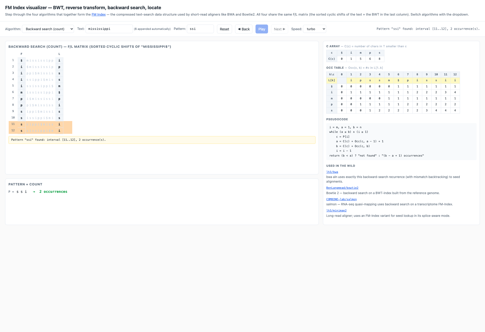
The right sidebar always shows the C array and the Occ table with the currently-consulted cells highlighted in orange. The active line of the pseudocode lights up yellow. The bottom yellow strip spells out the arithmetic for the current step.
Pairwise alignment — alignment/
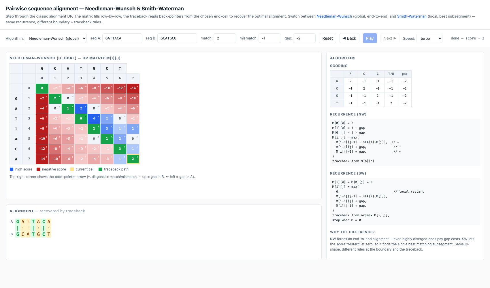
Side-by-side Needleman-Wunsch (global, end-to-end) and Smith-Waterman (local, best subsegment). Same DP shape — only the boundary conditions and traceback rules differ. Each cell shows its score and a back-pointer (↖ / ↑ / ←); the chosen traceback path is highlighted in green and the recovered alignment is rendered below the matrix with match/mismatch colouring.
Evoformer block — evoformer/
3-D voxel-grid walkthrough of one Evoformer block from AlphaFold 2. Each cube is one tensor cell; hue runs blue (negative) → red (positive). Use prev / next / play to step through MSA-row attention → MSA-column attention → outer product mean → triangle attention → triangle multiplication → transition.
This was already a self-contained tool in albi_exams/evoformer_viz/web/;
copied here unchanged for hosting.
Protein structure-similarity scores — structure-scores/
Interactive playground for the four scores that compare predicted vs. experimental protein structures: GDT-TS, TM-score, GDT-HA, lDDT. Move the per-residue distance sliders, watch each score update in real time, and read the short intuition panel.
Already self-contained at albi_exams/structure_scores/; copied here.
Phylogenetics — phylo/
Python implementations of the lecture’s distance-based
(neighbor_joining.py, upgma.py) and parsimony (fitch.py,
sankoff.py) tree-reconstruction algorithms, plus the rendered
step-by-step PNG figures. Run e.g.
cd phylo
python3 -c "from neighbor_joining import neighbor_joining; import numpy as np
D = np.array([[0,5,9,9,8],[5,0,10,10,9],[9,10,0,8,7],[9,10,8,0,3],[8,9,7,3,0]], float)
nwk, steps = neighbor_joining(['A','B','C','D','E'], D)
print(nwk)"
# → ((C:4,(A:2,B:3):3):1,(D:2,E:1):1);
Each step in steps carries the current distance matrix, Q matrix,
which two clusters were joined, the new branch lengths, and the
growing Newick string — perfect raw material for a future interactive
NJ visualizer (TODO).
Controls (uniform across all interactive demos)
- Reset — rewind to before any step
- ◀ Back — undo one step
- Play — toggle auto-advance (becomes Pause)
- Next ▶ — advance one step
- ← / → keys — back / forward
- space — toggle play/pause
- Speed dropdown — slow / medium / fast / turbo
URL parameters work the same way: ?seq=...&autoplay=1&speed=2
(plus per-demo extras documented at the top of each index.html).
Running locally
git clone https://github.com/r-sayar/algbio-edu.git
cd algbio-edu
python3 -m http.server 8765
# open http://localhost:8765
All demos are static HTML/CSS/JS — no build step. The phylo/
scripts need numpy (and matplotlib for the figures, which are
already pre-rendered as PNGs).
Credits
- Algorithms follow the Hölzer / Backofen / Liebl WS 2024 ALBI lectures at FU Berlin.
- The “DP matrix + structure side by side” teaching layout is inspired by the Backofen Lab’s RNA-Playground.
- All JavaScript here is original; the Evoformer and structure-scores
pages were already self-contained tools in
albi_exams/and are hosted unchanged.